Next: The local approximation
Up: The theoretical model
Previous: Introduction
The state of a system of  particles with velocities
 and positions
 (
( )
is represented by a point in
)
is represented by a point in  -dimensional
 -space of positional and velocity variables. The
-particle distribution
-space of positional and velocity variables. The
-particle distribution
 is defined as
the probability to find the system in the volume element
is defined as
the probability to find the system in the volume element
 around
  and
and  at time
  .
.
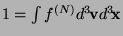
 is normalised as
 The evolution of the system is a trajectory in -space; the
evolution of a continuous subspace of systems at
The evolution of the system is a trajectory in -space; the
evolution of a continuous subspace of systems at  (initial conditions)
can be seen as a flow in -space, which due to the absence of
any dissipation is incompressible, and thus described by a
continuity equation in -space, which is Liouville's equation:
(initial conditions)
can be seen as a flow in -space, which due to the absence of
any dissipation is incompressible, and thus described by a
continuity equation in -space, which is Liouville's equation:
![\begin{displaymath}
\frac{\partial f^{(N)}}{\partial t} + \sum_{i=1}^N \Bigl\{
\...
...v}_i}
\Bigl[ f^{(N)} {d{\bf v}_i\over dt} \Bigr] \Bigr\} = 0 .
\end{displaymath}](img17.png) |
(1) |
Using the definition
 and
and
 , since
  and
and
 are independent coordinates, and if the forces are
conservative,
are independent coordinates, and if the forces are
conservative,
 ,
where
,
where  is the potential at the position of particle
  due
to the other particles, we can simplify last equation to
due
to the other particles, we can simplify last equation to
![\begin{displaymath}
\frac{\partial{f^{(N)}}}{\partial{t}} + \sum_{i=1}^N \Bigl[ ...
...
\frac{\partial{f^{(N)}}}{{\partial{\bf v}_i}} \Bigr] = 0 .
\end{displaymath}](img25.png) |
(2) |
Here it has been utilised that  does not depend on
itself, since the potential only depends on the
spatial coordinates.
does not depend on
itself, since the potential only depends on the
spatial coordinates.
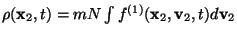
Now we introduce the one-particle distribution function
 as
as
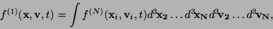 |
(3) |
the two-particle distribution function
 |
(4) |
and the two-particle correlation function  by
by
 |
(5) |
measures the excess probability of finding a particle at
 ,
,  due to the presence of another particle
at
due to the presence of another particle
at  ,
,  .
Since
.
Since  is normalised to
unity, one has
is normalised to
unity, one has
 ,
where
,
where  is a mean mass density, and
  the individual stellar mass.
Assuming that is symmetric with respect to exchange of
particles (i.e. all particles are indistinguishable), and observing that
the individual stellar mass.
Assuming that is symmetric with respect to exchange of
particles (i.e. all particles are indistinguishable), and observing that
 is also symmetric with respect to exchanges of the particles
  , one arrives at
 |
(6) |
Now one substitutes by the more common phase space density
 and drops for simplicity all subscripts ``1''. It
follows
and drops for simplicity all subscripts ``1''. It
follows
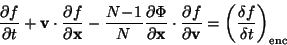 |
(7) |
If the average particle distance
 is bigger than
the impact parameter
is bigger than
the impact parameter  related to a
  deflection,
most of the scattering is due to small angle encounters, which change
velocity and position of the particle only weakly. So, if we assume that
all correlations stem from gravitational two-body scatterings of
particles, not from higher order correlations, we have that the Fokker-Planck
equation is
deflection,
most of the scattering is due to small angle encounters, which change
velocity and position of the particle only weakly. So, if we assume that
all correlations stem from gravitational two-body scatterings of
particles, not from higher order correlations, we have that the Fokker-Planck
equation is
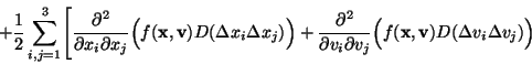
![\begin{displaymath}
+ {\partial^2\over\partial x_i\partial v_j}\Bigl(
f({\bf x...
...(
f({\bf x},{\bf v})
D(\Delta v_i\Delta x_j)\Bigr)
\Biggr] \
\end{displaymath}](img51.png) |
(8) |
Here the convenient notation of diffusion coefficients has been
introduced, which contain the integration over the velocity
and position changes, as e.g.:
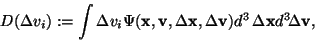 |
(9) |
where
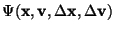
 is defined
as the probability for a star with position and velocity
to be scattered into a new phase space volume element
is defined
as the probability for a star with position and velocity
to be scattered into a new phase space volume element

 located around
 ,
,
 during the time interval
  .
.
Next: The local approximation
Up: The theoretical model
Previous: Introduction
Pau Amaro-Seoane
2005-02-25
![\begin{displaymath}
\bigg(\frac{\delta f}{\delta t}
\bigg)_{\rm enc}=
-\sum_{i...
...l(
f({\bf x},{\bf v})
D(\Delta v_i)\Bigr) \Biggr]
\nonumber
\end{displaymath}](img49.png)