There are two alternative ways of further simplification. One is the
orbit average, which uses that any distribution function, being a
steady state solution of the collisionless Boltzmann equation, can be
expressed as a function of the constants of motion of an individual
particle (Jeans' theorem). For the sake of simplicity, it is assumed
that all orbits in the system are regular, as it is the case for
example in a spherically symmetric potential; thus the distribution
function ![]() now only depends on maximally three independent integrals
of motion (strong Jeans' theorem). Let us transform the Fokker-Planck
equation to a new set of variables, which comprise the constants of
motion instead of the velocities
now only depends on maximally three independent integrals
of motion (strong Jeans' theorem). Let us transform the Fokker-Planck
equation to a new set of variables, which comprise the constants of
motion instead of the velocities ![]() . Since in a spherically
symmetric system the distribution only depends on energy and the
modulus of the angular momentum vector
. Since in a spherically
symmetric system the distribution only depends on energy and the
modulus of the angular momentum vector ![]() , the number of independent
coordinates in this example can be reduced from six to two, and all
terms in the transformed equation (8) containing derivatives to other
variables than
, the number of independent
coordinates in this example can be reduced from six to two, and all
terms in the transformed equation (8) containing derivatives to other
variables than ![]() and
and ![]() vanish (in particular those containing
derivatives to the spatial coordinates
vanish (in particular those containing
derivatives to the spatial coordinates ![]() ). Integrating the
remaining parts of the Fokker-Planck equation over the spatial
coordinates is called orbit averaging, because in our present example
(a spherical system) it would be an integration over accessible
coordinate space for given
). Integrating the
remaining parts of the Fokker-Planck equation over the spatial
coordinates is called orbit averaging, because in our present example
(a spherical system) it would be an integration over accessible
coordinate space for given ![]() and
and ![]() (which is a spherical shell
between
(which is a spherical shell
between
![]() and
and
![]() , the minimum and
maximum radius for stars with energy
, the minimum and
maximum radius for stars with energy ![]() and angular momentum
and angular momentum ![]() ).
Such volume integration is, since
).
Such volume integration is, since ![]() does not depend any more on
does not depend any more on
![]() carried over to the diffusion coefficients
carried over to the diffusion coefficients ![]() , which become
orbit-averaged diffusion coefficients.
, which become
orbit-averaged diffusion coefficients.
Orbit-averaged Fokker-Planck models treat very well the diffusion of orbits according to the changes of their constants of motion, taking into account the potential and the orbital structure of the system in a self-consistent way. However, they are not free of any problems or approximations. They require checks and tests, for example by comparisons with other methods, like the one described in the following.
We treat relaxation like the addition of a big non-correlated number
of two-body encounters. Close encounters are rare and thus we admit
that each encounter produces a very small deflection angle. Thence,
relaxation can be regarded as a diffusion process ![[*]](./footnote.png) .
.
A typical two-body encounter in a large stellar system takes place in
a volume whose linear dimensions are small compared to other typical
radii of the system (total system dimension, or scaling radii of
changes in density or velocity dispersion). Consequently, it is
assumed that an encounter only changes the velocity, not the position
of a particle. Thenceforth, encounters do not produce any changes
![]() , so all related terms in the Fokker-Planck equation
vanish. However, the local approximation goes even further and assumes
that the entire cumulative effect of all encounters on a test particle
can approximately be calculated as if the particle were surrounded by
a very big homogeneous system with the local distribution function
(density, velocity dispersions) everywhere. We are left with a
Fokker-Planck equation containing only derivatives with respect to the
velocity variables, but still depending on the spatial coordinates (a
local Fokker-Planck equation).
, so all related terms in the Fokker-Planck equation
vanish. However, the local approximation goes even further and assumes
that the entire cumulative effect of all encounters on a test particle
can approximately be calculated as if the particle were surrounded by
a very big homogeneous system with the local distribution function
(density, velocity dispersions) everywhere. We are left with a
Fokker-Planck equation containing only derivatives with respect to the
velocity variables, but still depending on the spatial coordinates (a
local Fokker-Planck equation).
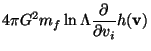
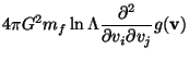
In practical astrophysical applications, the diffusion coefficients
occurring in the Fokker-Planck equation are not directly calculated,
containing the probability ![]() for a velocity change
for a velocity change
![]() from an initial velocity
from an initial velocity ![]() . Since
. Since ![]() , and
, and
![]() are of the dimension velocity
(change) per time unit, and squared velocity (change) per time unit,
respectively, one calculates such velocity changes in a more direct
way, considering a test star moving in a homogeneous sea of field
stars. Let the test star have a velocity
are of the dimension velocity
(change) per time unit, and squared velocity (change) per time unit,
respectively, one calculates such velocity changes in a more direct
way, considering a test star moving in a homogeneous sea of field
stars. Let the test star have a velocity ![]() and consider an
encounter with a field star of velocity
and consider an
encounter with a field star of velocity ![]() . The result of the
encounter (i.e. velocity changes
. The result of the
encounter (i.e. velocity changes ![]() of the test star) is
completely determined by the impact parameter
of the test star) is
completely determined by the impact parameter ![]() and the relative
velocity at infinity
and the relative
velocity at infinity
![]() ;
thus by an integration of the type
;
thus by an integration of the type
| (10) |
| (11) |
 |
|||
 |
(12) |
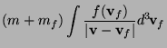 |
|||
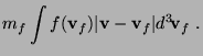 |
(13) |
![\begin{displaymath}
\bigg(\frac{\delta f}{\delta t}
\bigg)_{\rm enc}= -4\pi G^2...
...
{\partial^2 g \over\partial v_i\partial v_j}
\Bigr)\Biggr]
\end{displaymath}](img93.png) |
(14) |
Before going ahead the question is raised, why such approximation
can be reasonable, regarding the long-range gravitational force,
and the impossibility to shield gravitational forces as in the
case of Coulomb forces in a plasma by opposite charges. The key is
that logarithmic intervals in impact parameter ![]() contribute equally
to the mean square velocity change of a test particle,
provided
contribute equally
to the mean square velocity change of a test particle,
provided ![]() (see e.g. Spitzer87, chapter 2.1). Imagine that
on one hand side the lower limit of impact parameters (
(see e.g. Spitzer87, chapter 2.1). Imagine that
on one hand side the lower limit of impact parameters (![]() , the
, the
![]() deflection angle impact parameter) is small compared to
the mean interparticle distance
deflection angle impact parameter) is small compared to
the mean interparticle distance ![]() . Let on the other hand side
. Let on the other hand side
![]() be a typical radius connected with a change in density or
velocity dispersions (e.g. the scale height in a disc of a galaxy),
and
be a typical radius connected with a change in density or
velocity dispersions (e.g. the scale height in a disc of a galaxy),
and ![]() be the maximum total dimension of the system. Just to
be specific let us assume
be the maximum total dimension of the system. Just to
be specific let us assume ![]() , and
, and ![]() . In that case
the volume of the spherical shell with radius between
. In that case
the volume of the spherical shell with radius between ![]() and
and ![]() is
is ![]() times larger than the volume of the shell defined by
the radii
times larger than the volume of the shell defined by
the radii ![]() and
and ![]() . Nevertheless the contribution of both shells
to diffusion coefficients or the relaxation time is approximately
equal. This is a heuristic illustration why the local approximation
is not so bad; the reason is with other words that there are a lot
more encounters with particles in the outer, larger shell, but the
effect is exactly compensated by the larger deflection angle for
encounters happening with particles from the inner shell.
If we are in the core or in the plane of a galactic disc the density
would fall off further out, so the actual error will be smaller than
outlined in the above example. By the same reasoning one can
see, however, that the local approximation for a particle in a
low-density region, which suffers from relaxation by a nearby
density concentration, is prone to failure.
. Nevertheless the contribution of both shells
to diffusion coefficients or the relaxation time is approximately
equal. This is a heuristic illustration why the local approximation
is not so bad; the reason is with other words that there are a lot
more encounters with particles in the outer, larger shell, but the
effect is exactly compensated by the larger deflection angle for
encounters happening with particles from the inner shell.
If we are in the core or in the plane of a galactic disc the density
would fall off further out, so the actual error will be smaller than
outlined in the above example. By the same reasoning one can
see, however, that the local approximation for a particle in a
low-density region, which suffers from relaxation by a nearby
density concentration, is prone to failure.
These rough handy examples should illustrate that under certain conditions the local approximation is not a priori bad. On the other hand, it is obvious from our above arguments, that if we are interested in relaxation effects on particles in a low-density environment, whose orbit occasionally passes distant, high-density regions, the local approximation could be completely wrong. One might think here for example of stars on radially elongated orbits in the halo of globular clusters or of stars, globular clusters, or other objects as massive black holes, on spherical orbits in the galactic halo, passing the galactic disc. In these situations an orbit-averaged treatment seems much more appropriate.