In this section we introduce the fundamentals of the numerical
method we use to model our system. We give a brief description of the
mathematical basis of it and the physical idea behind it. The system
is treated as a continuum, which is only adequate for a large number
of stars and in well populated regions of the phase space. We consider
here spherical symmetry and single-mass stars. We handle relaxation in
the Fokker-Planck approximation, i.e. like a diffusive process
determined by local conditions. We make also use of the hydrodynamical
approximation; that is to say, only local moments of the velocity
dispersion are considered, not the full orbital structure. In
particular, the effect of the two-body relaxation can be modelled by a
local heat flux equation with an appropriately tailored conductivity.
Neither binaries nor stellar evolution are included at the presented
work. As for the hypothesis concerning the BH, see section
(![[*]](./crossref.png) ).
).
For our description we use polar coordinates, ![]()
![]() ,
, ![]() .
The vector
.
The vector
![]() denotes the velocity in
a local Cartesian coordinate system at the spatial point
denotes the velocity in
a local Cartesian coordinate system at the spatial point
![]() . For succinctness, we shall employ the notation
. For succinctness, we shall employ the notation
![]() ,
, ![]() ,
, ![]() . The distribution function
. The distribution function ![]() , is a
function of
, is a
function of ![]() ,
, ![]() ,
, ![]() ,
, ![]() only due to spherical symmetry,
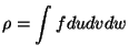
and is normalised according to
only due to spherical symmetry,
and is normalised according to
(r,t) = f(r,u,v^2+w^2,t) dudvdw.
Here ![]() is the mass density; if
is the mass density; if ![]() denotes the
stellar mass, we get the particle density
denotes the
stellar mass, we get the particle density
![]() . The
Euler-Lagrange equations of motion corresponding to the Lagrange
function
. The
Euler-Lagrange equations of motion corresponding to the Lagrange
function
L = 12(r^2 + r^2.^2 + r^2 ^2 .^2) - (r,t)
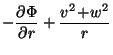
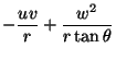
are the following
And so we get a complete local Fokker-Planck equation,
ft+v_rfr+v_r fv_r+v_f v_+v_fv_= ( ft )_FP
In our model we do not solve the equation directly; we use a so-called
momenta process. The momenta of the velocity distribution
function ![]() are defined as follows
are defined as follows
<i,j,k>:=^+_- v^i_r v^j_ v^k_ f(r, v_r, v_,v_,t)dv_rdv_dv_;
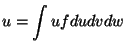
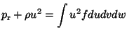
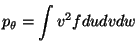
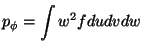
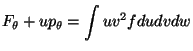
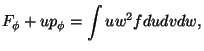
We define now the following moments of the velocity distribution function,
where ![]() is the density of stars,
is the density of stars, ![]() is the bulk velocity,
is the bulk velocity,
![]() and
and ![]() are the radial and tangential flux velocities,
are the radial and tangential flux velocities,
![]() and
and ![]() are the radial and tangential pressures,
are the radial and tangential pressures, ![]() is the radial and
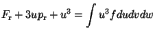
is the radial and ![]() the tangential kinetic energy flux
LS91. Note that the definitions of
the tangential kinetic energy flux
LS91. Note that the definitions of ![]() and
and ![]() are such
that they are proportional to the random motion of the stars. Due to
spherical symmetry, we have
are such
that they are proportional to the random motion of the stars. Due to
spherical symmetry, we have
![]() and
and
![]() . By
. By
![]() and
and
![]() the random velocity dispersions are given,
which are closely related to observable properties in stellar
clusters.
the random velocity dispersions are given,
which are closely related to observable properties in stellar
clusters.
![]() is a radial flux of random kinetic energy. In the
notion of gas dynamics it is just an energy flux. Whereas for the
is a radial flux of random kinetic energy. In the
notion of gas dynamics it is just an energy flux. Whereas for the
![]() and
and ![]() components in the set of Eqs.
(2.20) are equal in spherical symmetry, for the
components in the set of Eqs.
(2.20) are equal in spherical symmetry, for the ![]() and
and ![]() - quantities this is not true. In stellar clusters the
relaxation time is larger than the dynamical time and so any possible
difference between
- quantities this is not true. In stellar clusters the
relaxation time is larger than the dynamical time and so any possible
difference between ![]() and
and ![]() may survive many dynamical
times. We shall denote such differences anisotropy. Let us define the
following velocities of energy transport:
may survive many dynamical
times. We shall denote such differences anisotropy. Let us define the
following velocities of energy transport:
In case of weak isotropy (![]() =
=![]() )
) ![]() =
= ![]() , and thus
, and thus
![]() =
= ![]() , i.e. the (radial) transport velocities of radial and
tangential random kinetic energy are equal.
, i.e. the (radial) transport velocities of radial and
tangential random kinetic energy are equal.
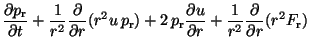
The Fokker-Planck equation (2.18) is multiplicated with various
powers of the velocity components ![]() ,
, ![]() ,
, ![]() . We get so up to
second order a set of moment equations: A mass equation, a continuity
equation, an Euler equation (force) and radial and tangential energy
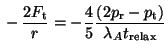
equations. The system of equations is closed by a phenomenological
heat flux equation for the flux of radial and tangential RMS ( root mean square) kinetic energy, both in radial direction. The
concept is physically similar to that of LBE80. The set of
equations is
. We get so up to
second order a set of moment equations: A mass equation, a continuity
equation, an Euler equation (force) and radial and tangential energy
equations. The system of equations is closed by a phenomenological
heat flux equation for the flux of radial and tangential RMS ( root mean square) kinetic energy, both in radial direction. The
concept is physically similar to that of LBE80. The set of
equations is
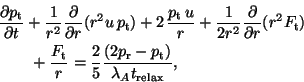
where ![]() is a numerical constant related to the time-scale of
collisional anisotropy decay. The value chosen for it has been
discussed in comparison with direct simulations performed with the
is a numerical constant related to the time-scale of
collisional anisotropy decay. The value chosen for it has been
discussed in comparison with direct simulations performed with the
![]() -body code GS94. The authors find that
-body code GS94. The authors find that ![]() is the physically realistic value inside the half-mass radius for all
cases of
is the physically realistic value inside the half-mass radius for all
cases of ![]() , provided that close encounters and binary activity do
not carry out an important role in the system, what is, on the other
hand, inherent to systems with a big number of particles, as this is.
, provided that close encounters and binary activity do
not carry out an important role in the system, what is, on the other
hand, inherent to systems with a big number of particles, as this is.
With the definition of the mass ![]() contained in a sphere of radius
contained in a sphere of radius
![]()
the set of Eqs.(2.22) is equivalent to gas-dynamical
equations coupled with the equation of Poisson. To close it we need an
independent relation, for moment equations of order ![]() contain
moments of order
contain
moments of order ![]() . For this intent we use the heat conduction
closure, a phenomenological approach obtained in an analogous way to
gas dynamics. It was used for the first time by [Lynden-Bell and Eggleton, 1980] but
restricted to isotropy. In this approximation one assumes that heat
transport is proportional to the temperature gradient,
. For this intent we use the heat conduction
closure, a phenomenological approach obtained in an analogous way to
gas dynamics. It was used for the first time by [Lynden-Bell and Eggleton, 1980] but
restricted to isotropy. In this approximation one assumes that heat
transport is proportional to the temperature gradient,
That is the reason why such models are usually also called conducting gas sphere models.
It has been argued that for the classical approach
![]() , one has to choose the Jeans'
length
, one has to choose the Jeans'
length
![]() and the standard
Chandrasekhar local relaxation time
and the standard
Chandrasekhar local relaxation time
![]() LBE80, where
LBE80, where ![]() is the mean free path
and
is the mean free path
and ![]() the collisional time. In this context we obtain a
conductivity
the collisional time. In this context we obtain a
conductivity
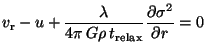
![]() . We shall consider this as
a working hypothesis. For the anisotropic model we use a mean velocity
dispersion
. We shall consider this as
a working hypothesis. For the anisotropic model we use a mean velocity
dispersion
![]() for the temperature
gradient and assume
for the temperature
gradient and assume
![]() BS86.
Forasmuch as, the equations we need to close our model are
BS86.
Forasmuch as, the equations we need to close our model are